Perceptron Model Explained

Introduction: The Simplest Brain-Inspired Model That Still Powers Modern AI

What if a machine could learn to make decisions using a process inspired by how neurons in the human brain work? The perceptron model is exactly that—one of the earliest and most fundamental building blocks of artificial intelligence. Despite its simplicity, it forms the conceptual foundation of modern neural networks and deep learning systems. Whether you are a student stepping into machine learning or a professional revisiting the basics, understanding the perceptron gives you clarity on how machines classify, separate, and interpret data.

In this article, we will explore the perceptron model in depth, uncover how it works mathematically, understand decision boundaries, and examine its limitations and real-world applications. By the end, you will have both theoretical clarity and practical intuition.

What is a Perceptron Model?

The perceptron is a supervised learning algorithm used for binary classification tasks. It attempts to classify input data into one of two categories by learning a linear decision boundary.

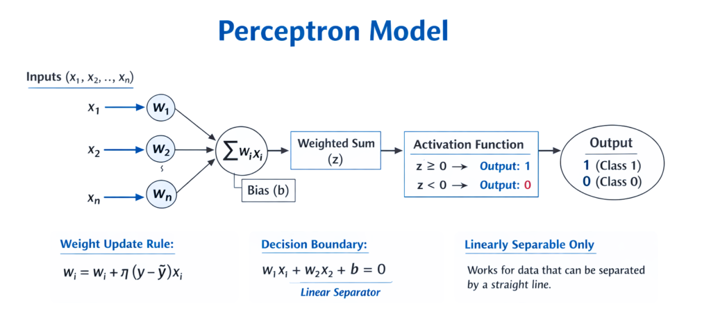
At its core, a perceptron mimics a biological neuron. It takes multiple inputs, applies weights to them, sums them up, and then passes the result through an activation function to produce an output.

Basic Components of a Perceptron

• Inputs (x₁, x₂, …, xₙ): Features of the dataset
• Weights (w₁, w₂, …, wₙ): Importance assigned to each feature
• Bias (b): Adjusts the decision threshold
• Activation Function: Determines the output (usually a step function)

The perceptron computes:$$z = w_1x_1 + w_2x_2 + \dots + w_nx_n + b$$

Then applies a step function:$$\text{Output} = \begin{cases} 1 & \text{if } z \geq 0 \\ 0 & \text{if } z < 0 \end{cases}$$Output={10​if z≥0if z<0​

This output represents the predicted class.

How the Perceptron Learns

The perceptron learns by adjusting weights based on prediction errors. This is done iteratively over the dataset.

Learning Rule (Weight Update Formula)

When the predicted output differs from the actual output, weights are updated as:$$w_i = w_i + \eta (y – \hat{y}) x_i$$

Where:

• η (eta) is the learning rate
• y is the actual label
• ŷ (y-hat) is the predicted label

This rule ensures that the model gradually improves its predictions.

Understanding Decision Boundaries

A decision boundary is the line (in 2D), plane (in 3D), or hyperplane (in higher dimensions) that separates different classes in the feature space.

Mathematical Interpretation

The decision boundary is defined by:$$w_1x_1 + w_2x_2 + b = 0$$

This equation represents a straight line in 2D.

Geometric Insight

• Points on one side of the boundary belong to class 1
• Points on the other side belong to class 0
• The boundary itself is where the model is uncertain

The perceptron essentially tries to find the best line that separates two classes.

Why Decision Boundaries Matter

Decision boundaries are critical because they define how a model distinguishes between categories. In the perceptron:

• The boundary is always linear
• It works well only if the data is linearly separable

This means you can draw a straight line to separate the classes.

Linear vs Non-Linear Data

Feature	Linearly Separable Data	Non-Linearly Separable Data
Definition	Data can be separated by a straight line	Requires curves or complex boundaries
Example	Height vs Weight classification	XOR problem
Perceptron Performance	Works well	Fails
Complexity	Simple	Complex

The perceptron struggles with problems like XOR, where no straight line can separate the data.

Step-by-Step Working of a Perceptron

1. Initialize weights and bias (usually small random values)
2. Take an input sample
3. Compute weighted sum
4. Apply activation function
5. Compare prediction with actual output
6. Update weights if error exists
7. Repeat for all data points (epochs)

This process continues until the model converges or reaches a stopping condition.

Python Implementation of Perceptron

Below is a simple implementation using NumPy:

import numpy as np# Step function
def step_function(z):
    return 1 if z >= 0 else 0# Training function
def train_perceptron(X, y, lr=0.1, epochs=10):
    weights = np.zeros(X.shape[1])
    bias = 0    for _ in range(epochs):
        for i in range(len(X)):
            z = np.dot(X[i], weights) + bias
            y_pred = step_function(z)
            
            error = y[i] - y_pred
            
            weights += lr * error * X[i]
            bias += lr * error    return weights, bias# Example dataset
X = np.array([[2, 3], [1, 1], [2, 1], [3, 2]])
y = np.array([1, 0, 0, 1])weights, bias = train_perceptron(X, y)print("Weights:", weights)
print("Bias:", bias)

This code trains a perceptron to classify simple data points.

Advantages of the Perceptron Model

1. Simplicity

The perceptron is easy to understand and implement, making it ideal for beginners.

2. Fast Computation

Since it uses linear operations, training is computationally efficient.

3. Foundation for Neural Networks

Modern deep learning models are built upon perceptron-like units.

Limitations of the Perceptron

1. Only Linear Decision Boundaries

It cannot handle complex, non-linear patterns.

2. Binary Classification Only

Standard perceptron works only for two classes.

3. Convergence Issues

If data is not linearly separable, the algorithm may never converge.

Perceptron vs Logistic Regression

Aspect	Perceptron	Logistic Regression
Output	Binary (0 or 1)	Probability (0 to 1)
Activation	Step function	Sigmoid function
Learning	Updates only on errors	Uses gradient descent
Decision Boundary	Linear	Linear
Interpretability	Low	Higher

Logistic regression is often preferred due to its probabilistic output and stability.

Real-World Applications of Perceptron

Although simple, perceptrons are used in:

• Spam detection systems
• Basic image classification
• Text sentiment classification
• Feature selection in pipelines

They are also stepping stones to more advanced models like multilayer neural networks.

From Perceptron to Deep Learning

The limitations of the perceptron led to the development of:

• Multi-Layer Perceptron (MLP)
• Neural Networks with hidden layers
• Deep Learning architectures

These models overcome linearity by introducing non-linear activation functions and multiple layers.

Key Intuition to Remember

Think of the perceptron as a line-drawing machine. It tries to draw a straight line that best separates two groups of points. If such a line exists, it will find it. If not, it struggles.

Conclusion

The perceptron model may appear simple, but its importance in the evolution of machine learning cannot be overstated. It introduces the fundamental idea of learning from data using weights and decision boundaries. While it has limitations, especially with non-linear data, it lays the groundwork for more complex models that dominate AI today.

Understanding the perceptron equips you with the intuition needed to grasp neural networks, optimization, and classification techniques. It is not just a historical model—it is a conceptual cornerstone.

---