Backpropagation Explained

Introduction: Why Backpropagation Is the Brain Behind Modern AI

If you’ve ever wondered how machines learn from mistakes the way humans do, backpropagation is the answer. It is not just another algorithm—it is the core mechanism that enables neural networks to improve, adapt, and eventually perform tasks like image recognition, language translation, and recommendation systems with remarkable accuracy. Every time a neural network makes a prediction and gets it wrong, backpropagation quietly steps in, calculates how wrong it was, and adjusts the system to perform better next time.

Despite its widespread use, backpropagation often feels intimidating because of its mathematical depth and layered structure. However, when broken down intuitively, it becomes a logical and elegant process. This article will walk you through both the intuition and mathematics of backpropagation, supported by examples, code, and comparisons, so you can build a strong conceptual and practical understanding.

What Is Backpropagation?

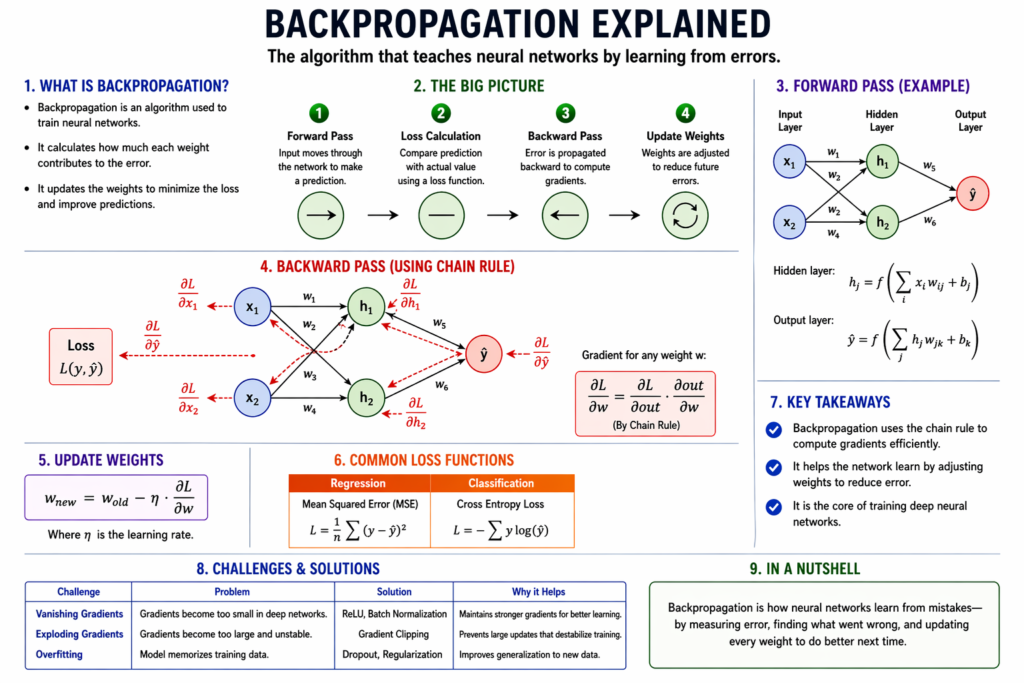
Backpropagation, short for “backward propagation of errors,” is an algorithm used to train neural networks by minimizing the difference between predicted outputs and actual outputs. It works by calculating gradients—essentially, how much each weight in the network contributes to the error—and then updating those weights to reduce future errors.

In simpler terms, backpropagation answers a key question:
“Which parts of the network are responsible for the mistake, and how should they change?”

The Intuition Behind Backpropagation

Imagine teaching a student to solve math problems. When the student gets an answer wrong, you don’t just say “incorrect”—you point out where they went wrong and guide them toward correction. Backpropagation works in a similar way.

Here’s the intuitive flow:

1. The network makes a prediction (forward pass).
2. The prediction is compared with the actual value (loss calculation).
3. The error is traced backward through the network (backward pass).
4. Each weight is adjusted slightly to reduce the error (optimization step).

The key idea is learning from mistakes by distributing responsibility across all layers of the network.

Understanding the Forward Pass

Before diving into backpropagation, it’s essential to understand the forward pass. In this phase:

• Inputs are fed into the network.
• Each layer processes the inputs using weights and activation functions.
• The final output is produced.

Mathematically, for a single neuron:$$z = w \cdot x + b$$$$a = f(z)$$

Where:

• $w$ = weights
• $x$ = input
• $b$ = bias
• $f$ = activation function
• $a$ = output

Loss Function: Measuring the Error

To improve, the model needs to know how wrong it is. This is done using a loss function.

For example, Mean Squared Error (MSE):$$L = \frac{1}{n} \sum (y_{true} – y_{pred})^2$$

This function quantifies the difference between actual and predicted values. The goal of training is to minimize this loss.

The Core Idea of Backpropagation

Backpropagation computes how much each weight contributes to the loss. It uses the chain rule from calculus to propagate the error backward.

The chain rule allows us to compute derivatives of composite functions:$$\frac{dL}{dw} = \frac{dL}{da} \cdot \frac{da}{dz} \cdot \frac{dz}{dw}$$

This tells us how a small change in a weight affects the final loss.

Step-by-Step Mathematical Breakdown

Let’s break down the process for a simple neural network:

Step 1: Compute Output Error

$$\text{Error} = y_{pred} – y_{true}$$

Step 2: Compute Gradient at Output Layer

$$\frac{\partial L}{\partial a} = 2 (y_{pred} – y_{true})$$

Step 3: Apply Chain Rule

$$\frac{\partial L}{\partial w} = \frac{\partial L}{\partial a} \cdot f'(z) \cdot x$$

Step 4: Update Weights

$$w = w – \eta \cdot \frac{\partial L}{\partial w}$$

Where:

• $\eta$= learning rate

This process is repeated for all layers, moving backward from output to input.

Why the Chain Rule Matters

The chain rule is what makes deep learning possible. Without it, calculating gradients across multiple layers would be computationally infeasible.

It ensures that:

• Each layer receives feedback proportional to its contribution to the error
• Learning is efficient even in deep networks

Gradient Descent and Optimization

Backpropagation works hand-in-hand with optimization algorithms like Gradient Descent.

Basic Gradient Descent Update Rule

$$\theta = \theta – \eta \cdot \nabla L$$

Where:

• $\theta$ = parameters (weights and biases)
• $\nabla L$ = gradient of loss

Types of Gradient Descent

Type	Description	Pros	Cons
Batch Gradient Descent	Uses entire dataset for each update	Stable convergence	Slow for large datasets
Stochastic Gradient Descent (SGD)	Updates per data point	Fast and efficient	Noisy updates
Mini-batch Gradient Descent	Uses small batches	Balance of speed and stability	Requires tuning batch size

A Simple Numerical Example

Let’s consider a single neuron:

• Input $x = 2$x=2
• Weight $w = 0.5$w=0.5
• Target $y = 4$y=4

Forward Pass:

$$y_{pred} = w \cdot x = 1$$

Loss:

$$L = (4 – 1)^2 = 9$$

Gradient:

$$\frac{dL}{dw} = -12$$

Update:

$$w = 0.5 – (0.1 \cdot -12) = 1.7$$

The weight increases, improving the prediction.

Python Code Example

Here’s a minimal implementation of backpropagation for a single neuron:

import numpy as np# Input and target
x = np.array([2])
y_true = np.array([4])# Initialize weight
w = np.array([0.5])
learning_rate = 0.1# Forward pass
y_pred = w * x# Loss
loss = (y_true - y_pred) ** 2# Backpropagation
grad = -2 * (y_true - y_pred) * x# Update
w = w - learning_rate * gradprint("Updated weight:", w)

This simple example demonstrates how gradients are computed and used to update weights.

Activation Functions and Their Role

Activation functions introduce non-linearity, allowing neural networks to learn complex patterns.

Function	Formula	Key Feature
Sigmoid	$\frac{1}{1+e^{-x}}$1+e−x1​	Smooth, bounded output
ReLU	$\max(0, x)$max(0,x)	Efficient and widely used
Tanh	$\tanh(x)$tanh(x)	Centered output

Backpropagation depends on derivatives of these functions, which is why differentiability is crucial.

Challenges in Backpropagation

1. Vanishing Gradient Problem

Gradients become extremely small in deep networks, slowing learning.

2. Exploding Gradient Problem

Gradients become too large, causing instability.

3. Overfitting

Model memorizes training data instead of generalizing.

Solutions to These Challenges

Problem	Solution
Vanishing gradients	Use ReLU, Batch Normalization
Exploding gradients	Gradient clipping
Overfitting	Dropout, regularization

Backpropagation in Deep Learning Today

Modern frameworks like TensorFlow and PyTorch automate backpropagation using automatic differentiation. This allows developers to focus on designing models rather than computing gradients manually.

However, understanding backpropagation remains essential for:

• Debugging models
• Improving performance
• Designing custom architectures

Why Backpropagation Matters in Real-World Applications

Backpropagation powers a wide range of technologies:

• Image recognition systems
• Natural language processing models
• Recommendation engines
• Autonomous vehicles

Without it, modern AI would not exist in its current form.

Key Takeaways

• Backpropagation is the learning mechanism of neural networks.
• It uses the chain rule to compute gradients efficiently.
• It works with optimization algorithms like gradient descent.
• Understanding it helps in building better AI systems.

---