Gradient Descent in Deep Learning

Behind every recommendation system, voice assistant, fraud detection model, or self-driving algorithm lies a deceptively simple idea: optimization. Deep learning models don’t magically “learn”—they iteratively adjust themselves to minimize error. At the heart of this process sits gradient descent, an algorithm so fundamental that without it, modern artificial intelligence would not exist.

Yet, while many learners memorize its formula, fewer truly understand how it behaves, why it struggles, and how its variants dramatically improve performance. This article goes beyond surface-level explanations. It builds intuition, connects math to real-world training dynamics, and explores how different gradient descent variants solve practical problems like slow convergence, noisy updates, and large-scale data challenges.

If you are a student, data scientist, or AI enthusiast aiming to deeply understand optimization in neural networks, this guide will give you a structured and practical foundation.

What is Gradient Descent? (Core Idea Explained Simply)

Gradient descent is an iterative optimization algorithm used to minimize a loss (cost) function by updating model parameters in the direction of the steepest descent, i.e., the negative gradient.

At a high level:

A model makes predictions
The error (loss) is calculated
The algorithm computes how to adjust parameters to reduce this error
Parameters are updated step by step

Mathematical Representation

$\theta = \theta – \alpha \cdot \nabla J(\theta)$

Where:

$\theta$ = model parameters (weights)
$\alpha$ = learning rate
$\nabla J(\theta)$ = gradient of the loss function

Intuition

Imagine standing on a mountain in fog, trying to reach the lowest valley:

You can’t see far ahead
You feel the slope beneath your feet
You take steps downhill

That “feeling of slope” is the gradient.

Why Gradient Descent is Crucial in Deep Learning

Deep learning models often have:

Millions (or billions) of parameters
Complex, non-linear loss surfaces
High-dimensional optimization spaces

Gradient descent allows:

Efficient navigation of this space
Continuous improvement through backpropagation
Scalable training across datasets

Without gradient descent, training neural networks would be computationally infeasible.

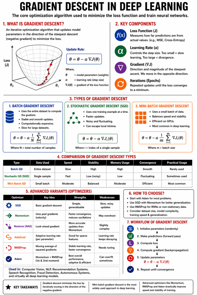
Key Components of Gradient Descent

1. Loss Function

Measures how far predictions are from actual values. Examples:

Mean Squared Error (MSE)
Cross-Entropy Loss

2. Learning Rate (α)

Controls step size:

Too small → slow learning
Too large → overshooting or divergence

3. Gradient

Represents the direction and magnitude of steepest ascent (we move opposite).

4. Iterations (Epochs)

Repeated updates until convergence.

Types of Gradient Descent

1. Batch Gradient Descent

How It Works

Uses the entire dataset to compute the gradient.

Characteristics

Stable and smooth updates
Computationally expensive
Slow for large datasets

Update Rule

$\theta = \theta – \alpha \cdot \frac{1}{N} \sum_{i=1}^{N} \nabla J(\theta)$

2. Stochastic Gradient Descent (SGD)

How It Works

Updates parameters using one data point at a time.

Characteristics

Faster updates
High variance (noisy)
Can escape local minima

3. Mini-Batch Gradient Descent

How It Works

Uses small batches of data (e.g., 32, 64, 128 samples).

Why It’s Popular

Balances speed and stability
Efficient on GPUs
Standard in deep learning

Comparison of Gradient Descent Types

Feature	Batch GD	Stochastic GD	Mini-Batch GD
Data Used	Entire dataset	Single sample	Small batch
Speed	Slow	Fast	Moderate
Stability	High	Low (noisy)	Balanced
Memory Usage	High	Low	Moderate
Convergence	Smooth	Fluctuating	Efficient
Practical Usage	Rare	Sometimes	Most common

Challenges with Basic Gradient Descent

Despite its simplicity, gradient descent faces real-world limitations:

1. Local Minima & Saddle Points

Models can get stuck in suboptimal regions.

2. Slow Convergence

Especially in flat regions or poorly scaled data.

3. Learning Rate Sensitivity

Choosing the wrong learning rate can break training.

4. Oscillations

In narrow valleys, updates may zig-zag.

Advanced Variants of Gradient Descent

To overcome these issues, several optimized versions were developed.

1. Momentum

Concept

Adds a fraction of previous updates to the current update.

Why It Helps

Accelerates convergence
Reduces oscillations

Formula

$v_t = \beta v_{t-1} + \alpha \nabla J(\theta)$ vt=βvt−1+α∇J(θ) $\theta = \theta – v_t$ θ=θ−vt

2. Nesterov Accelerated Gradient (NAG)

Concept

Looks ahead before calculating gradient.

Advantage

More accurate updates than momentum.

3. AdaGrad (Adaptive Gradient)

Concept

Adjusts learning rate for each parameter.

Strength

Works well for sparse data

Weakness

Learning rate keeps shrinking → stops learning

4. RMSProp

Concept

Fixes AdaGrad’s issue by using moving average of squared gradients.

Advantage

Stable learning rate
Faster convergence

5. Adam (Adaptive Moment Estimation)

Combines

Momentum (first moment)
RMSProp (second moment)

Why It Works Well

Adaptive learning rates
Fast convergence
Works well in most scenarios

Comparison of Gradient Descent Variants

Optimizer	Key Idea	Strengths	Weaknesses
SGD	Basic update	Simple, generalizable	Slow, noisy
Momentum	Uses past gradients	Faster convergence	May overshoot
NAG	Look-ahead gradient	More precise updates	Slightly complex
AdaGrad	Adaptive learning rate	Good for sparse features	Learning rate decay
RMSProp	Moving avg of gradients	Stable and efficient	Needs tuning
Adam	Momentum + RMSProp	Best overall performance	Can overfit sometimes

Python Implementation Example

Basic Gradient Descent

import numpy as np# Simple function: f(x) = x^2
def gradient(x):
    return 2 * x# Initialize
x = 10
learning_rate = 0.1# Gradient Descent
for i in range(20):
    grad = gradient(x)
    x = x - learning_rate * grad
    print(f"Step {i}: x = {x}")

Using Gradient Descent in Deep Learning (PyTorch Example)

import torch
import torch.nn as nn
import torch.optim as optim# Dummy model
model = nn.Linear(1, 1)# Loss function
criterion = nn.MSELoss()# Optimizer (Adam)
optimizer = optim.Adam(model.parameters(), lr=0.01)# Training loop
for epoch in range(100):
    x = torch.randn(10, 1)
    y = 2 * x + 1    # Forward pass
    y_pred = model(x)
    loss = criterion(y_pred, y)    # Backpropagation
    optimizer.zero_grad()
    loss.backward()    # Update weights
    optimizer.step()    print(f"Epoch {epoch}, Loss: {loss.item()}")

How to Choose the Right Optimizer

General Guidelines

Start with Adam for most problems
Use SGD with Momentum for better generalization
Use RMSProp for RNNs or non-stationary data

Factors to Consider

Dataset size
Model complexity
Training speed
Generalization performance

Real-World Applications of Gradient Descent

Gradient descent is used in:

Image recognition (CNNs)
NLP models (Transformers)
Recommendation systems
Fraud detection
Autonomous driving systems

Essentially, every modern AI system relies on it.

Conclusion: Why Mastering Gradient Descent Matters

Gradient descent is not just an algorithm—it is the foundation of learning in machines. Understanding its behavior, limitations, and variants allows you to:

Train models more efficiently
Debug convergence issues
Improve performance significantly

While tools like PyTorch and TensorFlow abstract much of the complexity, deeper understanding gives you an edge in both research and industry applications.