
Introduction: How Machines Finally Learned to Remember (and Why It Matters More Than Ever)
In the early days of deep learning, neural networks had a frustrating limitation: they could “see” patterns, but they struggled to remember them. Imagine trying to understand a sentence without recalling its beginning, or predicting stock prices without knowing yesterday’s trend. This is where Long Short-Term Memory (LSTM) networks transformed the landscape.
Designed to capture long-term dependencies in sequential data, LSTMs gave machines a structured way to remember what matters and forget what doesn’t. Today, they power everything from speech recognition and language translation to time-series forecasting and anomaly detection. In this article, we will explore how LSTM networks work, why they are so effective, and how they solve one of the most fundamental challenges in machine learning.
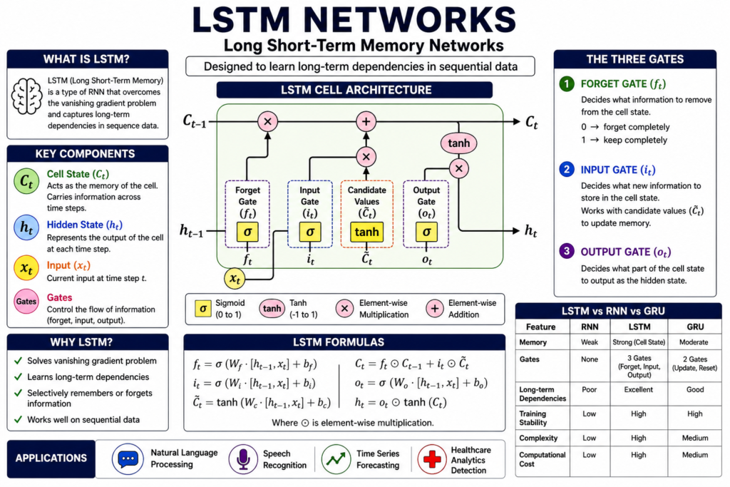
What Are LSTM Networks?
Long Short-Term Memory (LSTM) networks are a special type of Recurrent Neural Network (RNN) designed to handle sequential data and capture long-range dependencies. Unlike traditional feedforward neural networks, which process inputs independently, LSTMs maintain a memory of past information through time.
At their core, LSTMs are built to overcome the limitations of standard RNNs, particularly the vanishing gradient problem, which makes it difficult for networks to learn from long sequences. By introducing a carefully designed memory mechanism, LSTMs can retain relevant information over extended time steps, making them highly effective for tasks involving sequences such as text, speech, and time-series data.
Why Traditional RNNs Struggle with Long-Term Dependencies
Before understanding LSTMs, it is important to recognize the problem they solve. Standard RNNs process sequences step by step, passing hidden states forward. However, during training, gradients used to update weights tend to shrink (vanish) or grow uncontrollably (explode).
This leads to two key issues:
- Vanishing gradients: The network forgets earlier information in long sequences.
- Exploding gradients: Training becomes unstable due to excessively large updates.
As a result, traditional RNNs are good at capturing short-term patterns but fail to retain long-term dependencies, such as the context in a long paragraph or trends in long time-series data.
How LSTM Networks Solve the Memory Problem
LSTM networks introduce a cell state and a set of gates that regulate the flow of information. This architecture allows the model to selectively remember or forget information over time.
Key Components of an LSTM Cell
An LSTM cell consists of:
- Cell State (Cₜ)
This acts as the memory of the network. It carries information across time steps with minimal modification, allowing long-term dependencies to persist. - Hidden State (hₜ)
This represents the output at each time step and is used for predictions. - Gates
Gates are neural networks that control information flow. They use sigmoid activation to decide what to keep or discard.
Understanding the Three Gates in LSTM
1. Forget Gate
The forget gate determines what information should be discarded from the cell state. It looks at the previous hidden state and the current input and outputs a value between 0 and 1.
- 0 → Completely forget
- 1 → Completely retain
This mechanism ensures that irrelevant or outdated information is removed.
2. Input Gate
The input gate decides what new information should be added to the cell state. It works in two steps:
- A sigmoid layer determines which values to update.
- A tanh layer creates candidate values.
These are combined to update the memory selectively.
3. Output Gate
The output gate determines what information from the cell state should be used to produce the output. It filters the memory and generates the hidden state for the current time step.
Mathematical Intuition Behind LSTM
The LSTM operations can be summarized as follows:
- Forget gate:
- Input gate:
- Candidate memory:
- Cell state update:
- Output gate:
- Hidden state:
This design allows LSTMs to maintain stable gradients during training, enabling them to learn long-term relationships effectively.
Why LSTMs Are Effective for Long-Term Dependencies
LSTMs manage long-term dependencies through:
- Controlled memory flow: Gates regulate what information enters and leaves memory.
- Constant error flow: The cell state allows gradients to pass unchanged over time.
- Selective forgetting: Irrelevant data is removed, preventing noise accumulation.
This combination ensures that important information persists across many time steps without degradation.
LSTM vs RNN vs GRU: A Comparative Overview
| Feature | RNN | LSTM | GRU |
|---|---|---|---|
| Memory Handling | Limited | Strong long-term memory | Moderate memory |
| Gates | None | 3 (Input, Forget, Output) | 2 (Update, Reset) |
| Complexity | Low | High | Medium |
| Training Stability | Poor | Stable | More stable than RNN |
| Performance on Long Data | Weak | Strong | Strong |
| Computational Cost | Low | High | Lower than LSTM |
While LSTMs are powerful, GRUs are often used as a simpler alternative with comparable performance in many tasks.
Real-World Applications of LSTM Networks
LSTMs have become a foundational model for sequence-based tasks across industries:
1. Natural Language Processing (NLP)
Used in language modeling, text generation, and machine translation.
2. Speech Recognition
Helps systems understand spoken language by analyzing temporal audio patterns.
3. Time-Series Forecasting
Used in stock price prediction, weather forecasting, and demand forecasting.
4. Healthcare Analytics
Analyzes patient data sequences for diagnosis and prediction.
5. Anomaly Detection
Identifies unusual patterns in sequential data such as fraud detection.
Simple LSTM Implementation in Python
Below is a basic example using TensorFlow/Keras:
import numpy as np
from tensorflow.keras.models import Sequential
from tensorflow.keras.layers import LSTM, Dense

# Sample dataset
X = np.array([[1, 2, 3], [2, 3, 4], [3, 4, 5]])
y = np.array([4, 5, 6])

# Reshape input to [samples, time steps, features]
X = X.reshape((X.shape[0], X.shape[1], 1))

# Build LSTM model
model = Sequential()
model.add(LSTM(50, activation='relu', input_shape=(3, 1)))
model.add(Dense(1))

model.compile(optimizer='adam', loss='mse')

# Train model
model.fit(X, y, epochs=200, verbose=0)

# Predict
pred = model.predict(X)
print(pred)
This example demonstrates how LSTM learns patterns in sequences and predicts future values based on past observations.
Advantages of LSTM Networks
- Capable of learning long-term dependencies
- Handles sequential data effectively
- Reduces vanishing gradient problem
- Highly versatile across domains
Limitations of LSTM Networks
- Computationally expensive
- Requires large datasets for optimal performance
- Slower training compared to simpler models
- Can be overkill for short sequences
When Should You Use LSTM?
You should consider using LSTM when:
- Your data is sequential or time-dependent
- Long-term dependencies are important
- Context matters across many time steps
However, for simpler problems or shorter sequences, alternatives like GRU or even traditional machine learning models may be more efficient.
The Future of LSTMs in the Age of Transformers
While LSTMs were once the dominant architecture for sequence modeling, newer models like Transformers have gained popularity due to their ability to process sequences in parallel and capture global dependencies more efficiently.
However, LSTMs still remain relevant, especially in:
- Low-resource environments
- Real-time systems
- Edge devices with limited computational power
Their simplicity and interpretability continue to make them valuable in many practical applications.